A Simple Approach to Using LLMs for Missing Data
Author: James Brand
Date: 2025-07-14
This post is a short outline of an idea I tested with Mert Demirer. We worked together to write this up here as well. So, the writing here will be a combination of “my” and “our” opinions and pronouns.
The main idea in this post is that LLMs have a lot of knowledge about the world, and that this knowledge might be useful for imputing missing data. There are some papers already out there discussing LLMs and imputation, but the ones I’ve seen (e.g., 1, 2, 3) either treat the LLM imputation as competing with standard in-sample imputation or focus on fine-tuning/training custom LLMs. Instead, we ask whether an off-the-shelf LLM can provide a useful signal beyond the data you already have. As we’ll discuss below, testing this is easy and cheap to do in any setting, and I’m surprised it hasn’t been done more broadly already.
Background and method
Querying LLMs for factual knowledge
In 2023, I wrote a paper with Ayelet Israeli and Donald Ngwe, where we showed that you can ask an LLM survey questions as if it were a human and it answers like real humans in many ways. There are many papers showing similar things in other contexts (notably John Horton’s earlier paper, but many others since). Although I’m still bullish on this, lots of critiques of the paper call out that you can’t know whether any given LLM simulation is accurate; no matter how many tests you do, at some point you’re “trusting” that the LLM can simulate people in a new setting
I think the issue is just that we started more ambitiously than we needed to. Before creating brand new simulated datasets from LLMs, we could instead use LLMs to supplement incomplete datasets. If the LLM has “learned” real world correlations, then it could be pretty good at this. Imagine I have a market research survey with respondents’ demographics, but some participants chose not to report their income. However, imagine that in other parts of the survey they described major purchases they’ve made in the past (“Last year I purchased a new Whirlpool washer and a Tesla”). With normal imputation tools, it would be difficult to use the latter to impute income. With an LLM, in contrast, it’s straightforward in theory; you can just describe or list qualitative features and ask for the LLM’s best guess.
Our approach to LLM-augmented imputation
The precise approach we’ll take is this: we’ll use an LLM to predict all values of a single column in a dataset, and then use non-missing rows to estimate weights to combine (a) LLM-generated signals and (b) standard in-sample imputations into an ensemble imputation.
The idea is simple. Take a dataset which has some missing values for column B, but where column A is never missing. Then,
- Baseline Imputation Generate an initial imputation using standard methods. This could be via OLS or any other off-the-shelf imputation method.
- LLM Imputation Using rows for which neither A nor B are missing, use the LLM to impute values of B as a function of A (one proposal below)
- Ensemble weights/Cross-Validation Partition the data into test and evaluation sets. Use the test set to develop weights for the two methods (LLM and standard imputation) to maximize a validation metric (e.g., out of sample accuracy on known values of column B)
- Prediction Use the estimated ensemble weights to combine available signals into final imputation on missing rows
In essence: generate imputations from an LLM in your preferred way (or many ways all at once!), and then treat those imputations, as well as any you can generate using in-sample variation, as imputation “models” in a very standard ensemble setup. Then, you simply estimate weights (again, however you prefer) to determine how to combine these models effectively. This can be done quickly via OLS or through any number of nonlinear methods in the ensembling literature.
Testing LLM-augmented imputation
For testing, we pulled the third quarter of fiscal year 2021 from the Compustat dataset (financial reports). For each row of our dataset, we gave an LLM a string indicating the name and COGS (cost of goods sold) of the company, asking it to predict the company’s revenue. The exact prompt we used for this test is the following (though other variants performed pretty similarly):
“You are an expert data imputation AI tool. Users will provide pieces of information about a row of a dataset which is missing a field, and your job is to provide the best possible prediction for the missing field. You use all available information both within the prompt and from your own experience and knowledge to make the best possible prediction. Your answer should be a single number, with no extraneous symbols or additional words.
Description: A firm was randomly selected from a dataset detailing the quarterly financial records of all publicly traded firms.
Precise data for this randomly selected firm in the third quarter of fiscal year 2021 is as follows:
Cost of Goods Sold (Millions): $ (COGS)
Company Name: (NAME)
Revenue (Millions): $”
Nothing complicated at all; we’re almost literally asking it to fill in the missing revenue data for us. You could do this for any dataset, any combination of missing fields, and of any format. You could easily add generic text columns here, which is part of the reason we include company name in the prompt.
We focus on two evaluation metrics:
In-sample prediction: we regress revenue on COGS (which we gave to the LLM), and then we regress revenue on both COGS and the LLM-generated signal. Comparing the adjusted R2 of these two regressions gives a sense of whether the LLM-generated signal is providing information beyond the data in the prompt.
Out-of-sample prediction: we estimate the combined regression (COGS + LLM) above on one random subset of the data, then use the coefficients from that regression to predict the missing variable on a holdout set. We then compare the predictions to the true values of the missing variable, and compute the correlation between them. We repeat this many times on different random cuts of the data and then compare the distributional performance of LLM-augmented predictions to OLS predictions alone.
Findings
We ended up testing the following combinations of models, temperature settings, and number of responses (averaged to calculate one LLM signal):
| Model | Temperature | Responses |
|---|---|---|
| gpt-4.1-nano | 0.0 | 1 |
| gpt-4.1-nano | 1.0 | 1 |
| gpt-4.1-nano | 1.0 | 10 |
| gpt-4.1-nano | 1.0 | 30 |
| gpt-4.1-mini | 1.0 | 30 |
| gpt-4.1 | 1.0 | 30 |
| o1 | 1.0 | 1 |
| o4-mini | 1.0 | 1 |
For each combination, we calculated out-of-sample predictions for 30,000 random partitions of the data, and our ensemble weights were calculated once for each partition using OLS.
Finding 1: GPT 4.1 adds a useful signal
The plot below shows the distribution of in-sample adjusted R2 when we impute revenue
via OLS using COGS, imputations from GPT 4.1, or both. Combining the two
signals gives us a better in-sample prediction than either alone, so as
a baseline the LLM-generated signal seems to contain something useful. I
think we’re even giving the LLM a hard problem here. Baseline R2 is already very high,
but still the LLM signal improves prediction considerably. 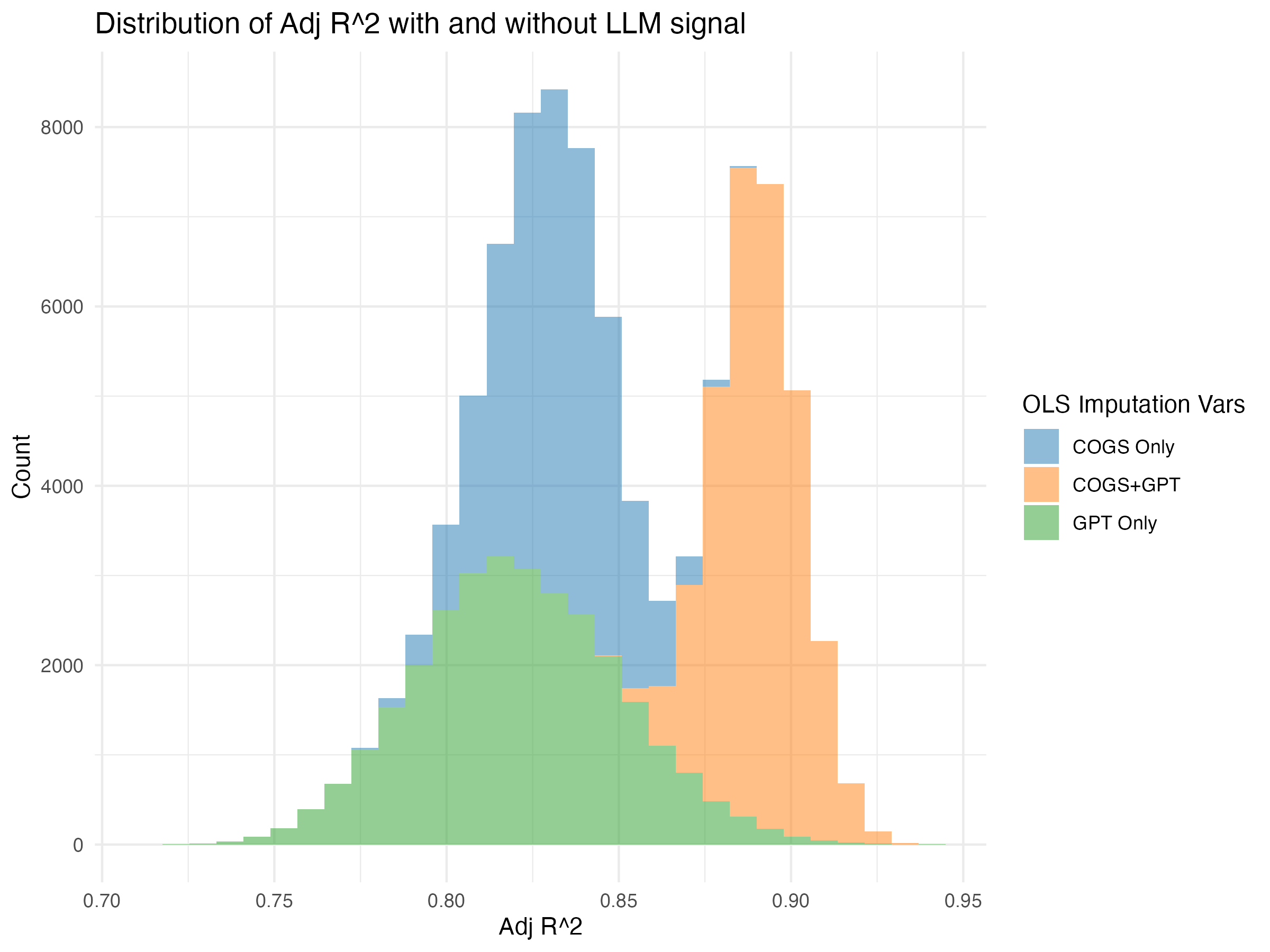
Finding 2: Diminishing returns to more responses
I mentioned above that we averaged over 30 responses for the GPT 4.1
model, but this was an arbitrary choice. We also tried, with
GPT-4.1-nano, comparing in-sample performance with a single response and
with 10-response averages. The plot below shows how 4.1-nano’s
performance varies as we average over more responses. Averaging 10
responses performs much better on average than 1, but 30 responses
doesn’t add much value. This was surprising to me, given the high
variance of raw responses, but I’m not sure I have enough intuition to
say much more than that. 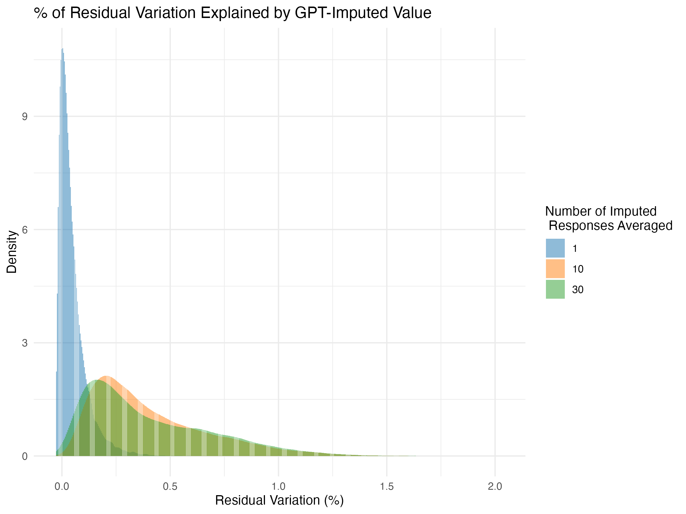
Finding 3: Bigger models are better
It turns out that all flagship LLMs are reasonably good at this
imputation problem, but bigger models are much better
than small ones. Continuing with the same type of plot, we can compare
the amount of residual in-sample variation explained across many models.
We find that both reasoning models are clearly better than the
non-reasoning models, and o1 is a clear winner. Moreover, GPT-4.1 far
outperforms its -mini and -nano variants. 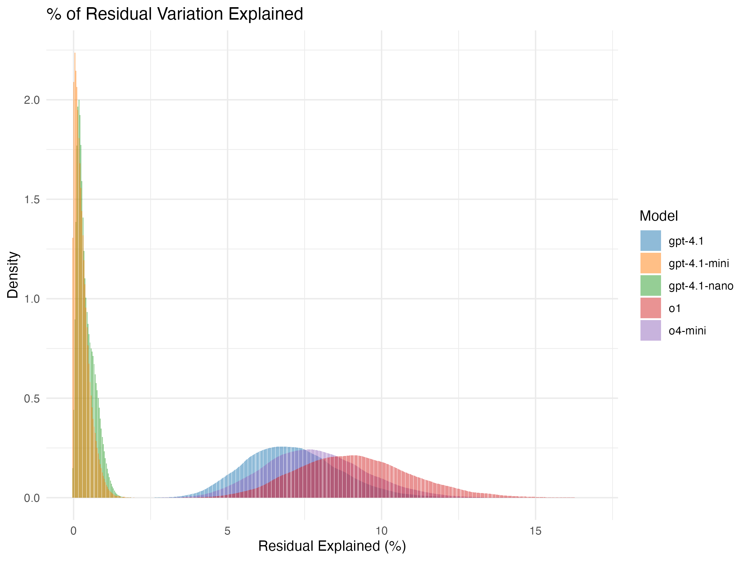
Finally, we look at out-of-sample performance, and
we find the same patterns as we did on in-sample metrics. First, we plot
the actual revenue values in our data against the imputations created by
OLS using COGS and LLM signals together. The zeros here are cases in
which we could not parse a number from the LLM’s response. 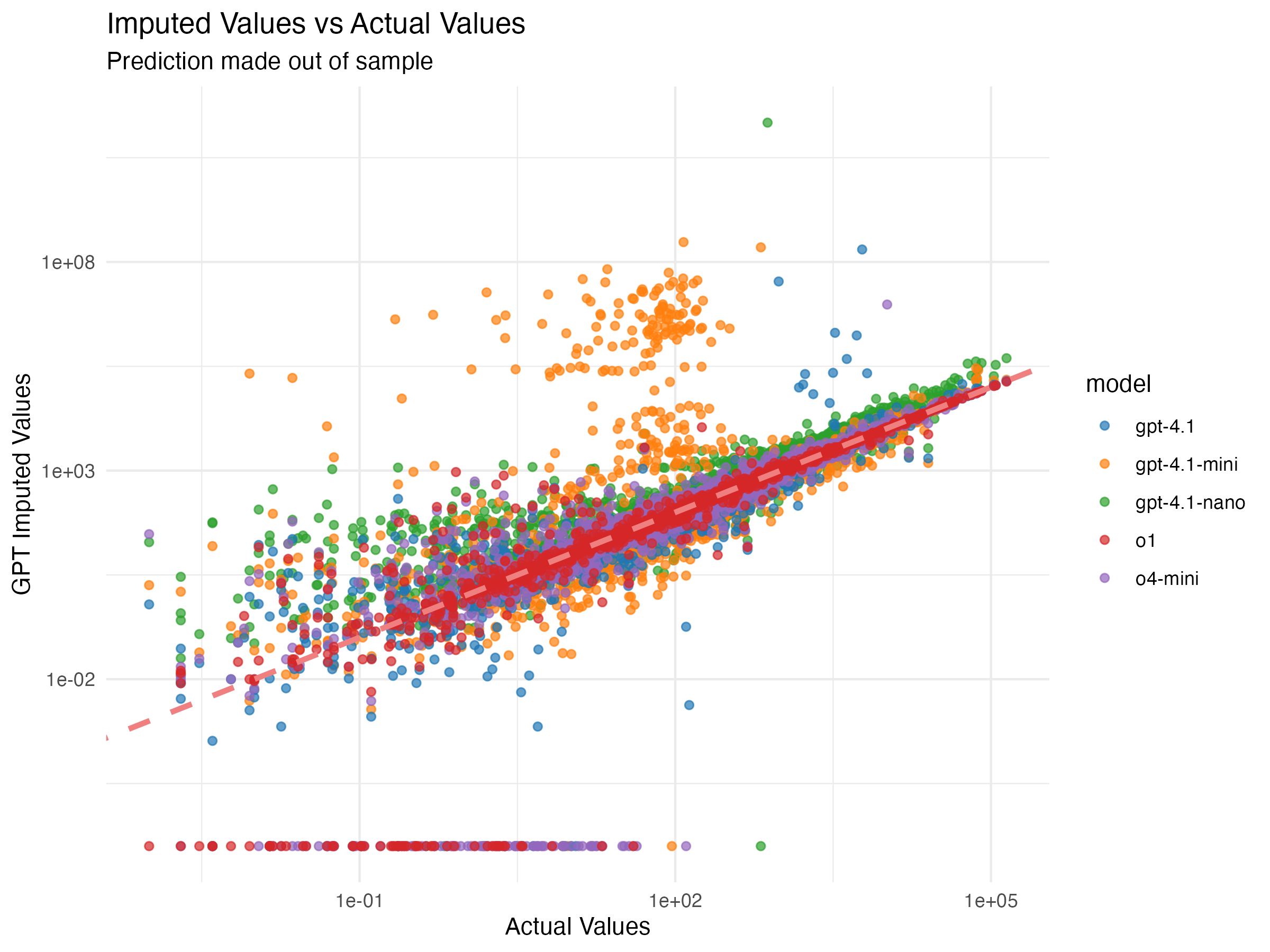
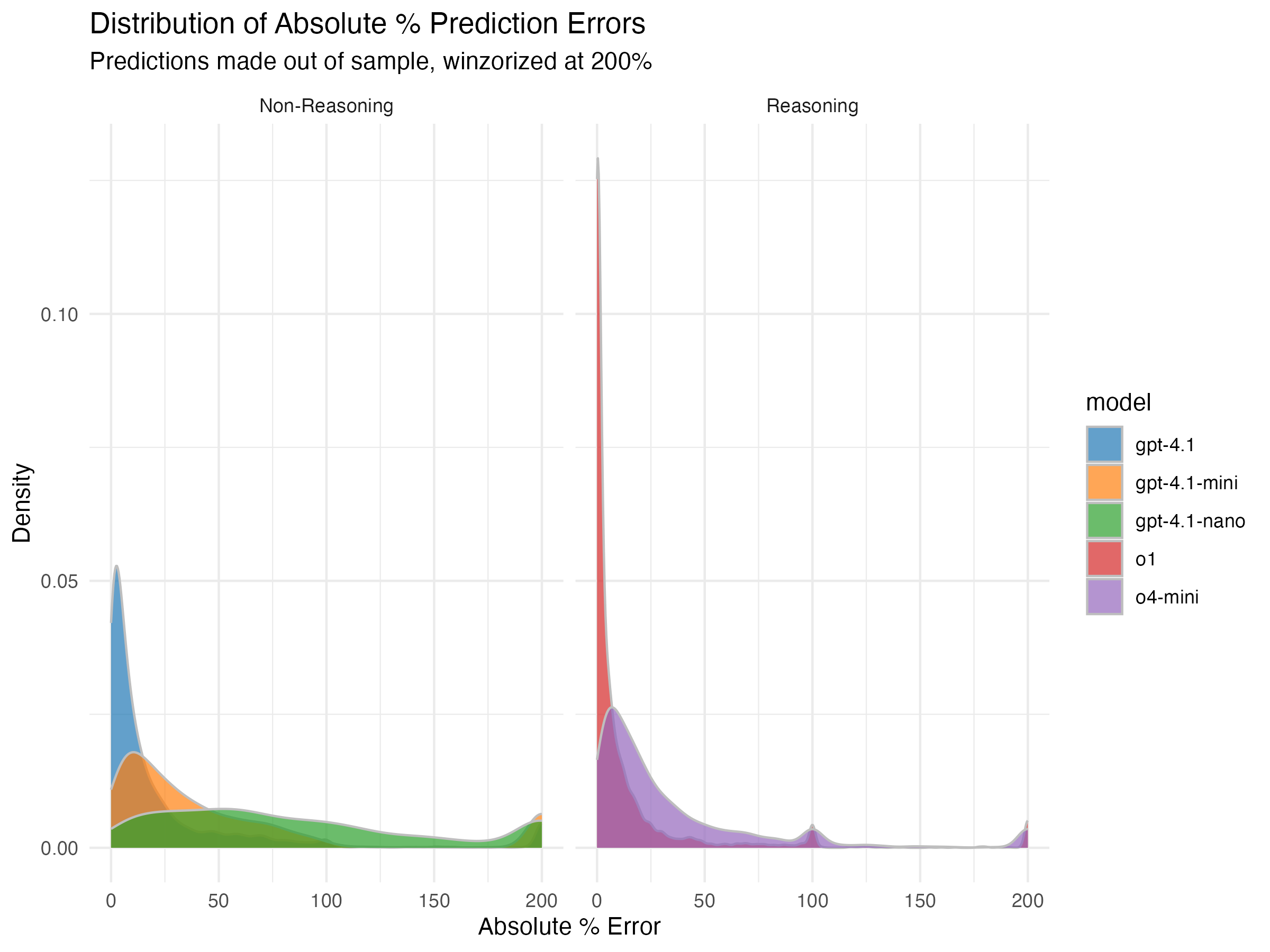
Finally, we can look directly at the out-of-sample prediction errors
directly. Here we see that o1 is just a far better predictor than the
rest of the imputations. Many of the other models frequently miss the
prediction target by over 50%, but o1 rarely missed by more than 25%.
What is perhaps surprising is that GPT-4.1 beats o4-mini. I don’t know
near enough about how “-mini” series LLMs are created to know for sure,
but I’m assuming it results in a significantly smaller model. In this
case, that seems to have hurt its productivity at this prediction task.
Takeaways and Caveats
Overall, the results here are pretty encouraging. LLMs add a useful signal beyond the in-sample data. Now for the caveats:
OLS imputation is simplistic. We could expand this to more sohpisticated methods, which could reduce the incremental value of the LLM-generated signal.
This approach won’t help in every dataset. You might have enough non-missing data to impute with high confidence without an LLM, or there may not be LLMs with enough context for your setting to provide a useful signal.
Cost was a bigger concern than I expected. The costs of GPT 4.1-nano and -mini were trivial, but for the larger and more performant models it cost multiple dollars to impute a few thousand rows of data for one variable. There are various ways to be more token-efficient than we were, and these costs continue to plummet, but it is definitely a short-run limitation to consider.
On a more optimistic concluding note, LLMs “know” a lot, and all we need here is that the LLM provides some sort of independent signal not captured by the available data. If we have that, then we can probably do some version of this cross-validation ensemble weight estimation. This is importantly different from the way imputation usually works, where we are using in-sample variation in increasingly clever ways, and thus don’t really gain any new data/power via the imputation itself. The nice thing here is that the method is, statistically speaking, nearly “free”, because you can learn the best weights to assign to the LLM-generated signal in the ensemble step. So, as long as your data has enough non-missing rows to learn these weights, you can use the LLM-generated signal without worrying too much about whether the LLM is “right” or “wrong” in some absolute sense.